 Nawaz Labs
Training a Custom Earlobe Keypoint Tracker for Browser-Based Earring Try-On, and What Perfection Costs
Research Note 001 · v0.1 draft for review
Nawaz Pasha · 5 July 2026 · 12 min read
Abstract
Virtual earring try-on lives or dies on one anatomical point: the piercing point on the earlobe. No general-purpose browser landmark model provides it. This note documents two things. First, the tracking stack that ships today on a production jewellery try-on platform (a purpose-built ear detection network, geometric interpolation, adaptive smoothing, and an optical-flow fallback) and its measured limits. Second, an end-to-end experiment answering the question those limits raise: can we train our own lobe-specific model, deployable in the browser, without a research team?
The experiment produced a six-phase pipeline, built and run in a single day: video capture → frame extraction → web-based labeling → YOLO-pose fine-tuning → verified ONNX export → an npm package. The checkpoint itself is deliberately narrow, a single-subject proof. The pipeline is the result: it converts recorded video into tracker accuracy mechanically, so scaling to a production-grade tracker stops being a research question and becomes a data-collection program with a known price. The final section specifies that program: capture protocol, ear-type coverage, annotation effort, and compute, each derived from a measured anchor in this run.
1 · The problem: one point decides realism
An earring does not sit "on the ear." It hangs from the piercing point on the lobe, a region a few pixels wide in a webcam frame. Everything the try-on renders is anchored there:
- Placement. The jewellery sprite is drawn at that point; anchor error of a few pixels reads instantly as "stuck on, not worn."
- Physics. Hanging earrings on the platform are simulated as constraint chains (60 Hz, 16 constraint iterations per substep). The chain is pinned at the lobe anchor, so anchor jitter does more than move the earring: it injects energy into the simulation, and that energy multiplies down the chain as visible swinging the user never caused.
- The browser constraint. All of this must run client-side, with no server round-trips, at interactive frame rates on mid-range phones.
The difficulty is that the earlobe is a point almost no general model was trained to find:
| Model family | What it offers at the ear | Why it falls short |
|---|---|---|
| MediaPipe Face Landmarker | 478 facial landmarks, none on the lobe | Lobe must be derived from nearby geometry; ear coverage degrades sharply on profile views, exactly the pose earring try-on needs |
| COCO-style pose models | One "ear" keypoint | Located near the tragus, not the lobe; single point, no ear structure |
| WebAR.rocks ear network | Dedicated ear landmarks (earBottom, earEarring) | The best available, but generic: fixed weights, not retrainable, and the lobe still comes from interpolation, never from the model |
2 · What ships today (confirmed)
The production stack is the strongest configuration we found without training anything:
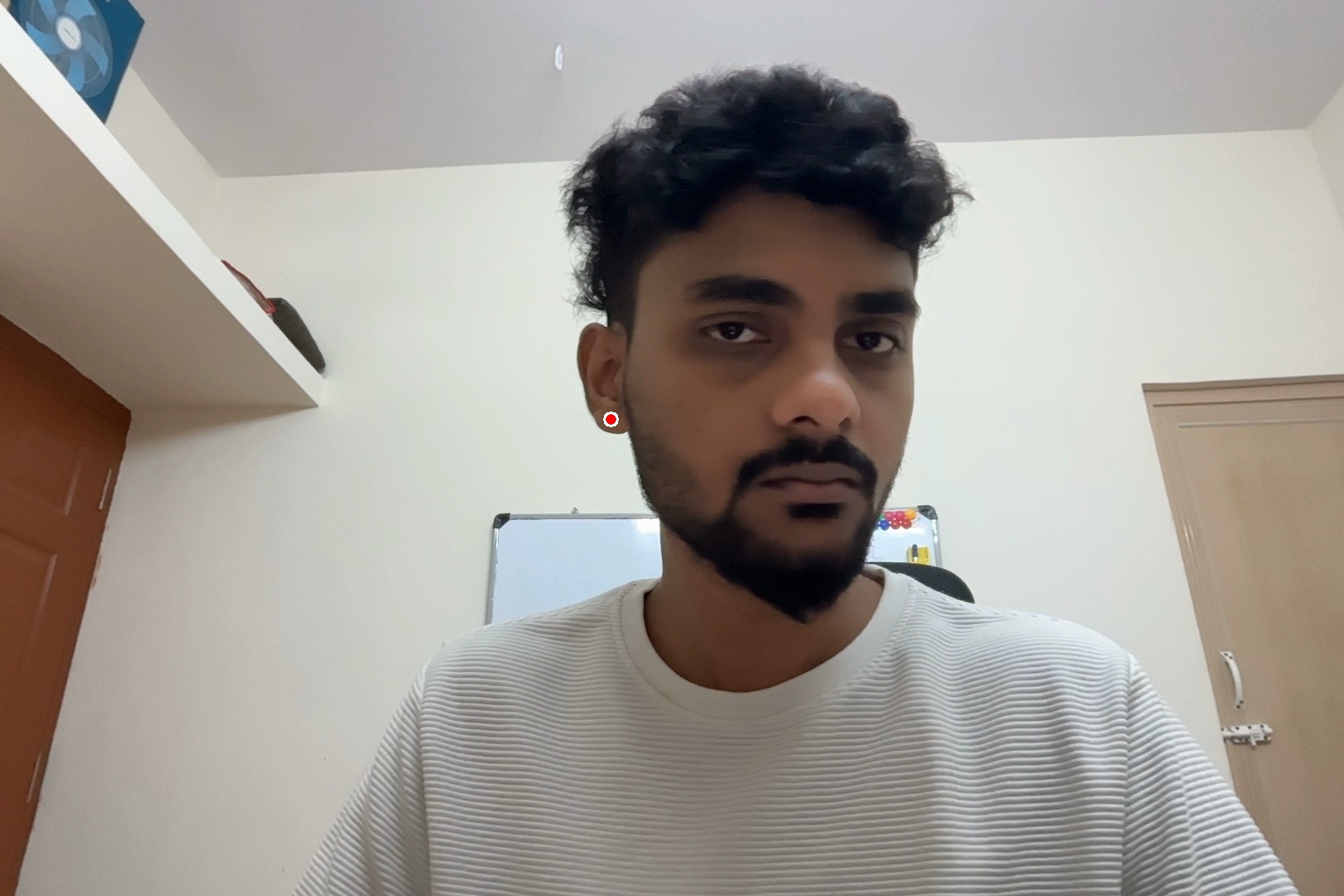
drop at public/research/earlobe-tracker/media/current-tracker-points.mp4drop at public/research/earlobe-tracker/media/current-tracker-limits.jpgIts properties, in production terms:
- What it does well. Stable enough to ship: it anchors a catalog of 27 tryable earrings, including chain-physics pieces, across desktop and mobile. The optical-flow fallback (with forward-backward validation to reject the classic silent Lucas-Kanade failure) keeps tracking alive on extreme close-ups where the face network loses lock.
- Where it stops. The lobe is derived, not learned: a fixed interpolation constant plus per-device nudge factors, tuned by hand and clamped to keep multi-device parity. It drifts on extreme poses; the underlying network is a black box we cannot retrain when it's wrong; and every accuracy improvement so far has been smoothing and guarding around the anchor, never improving the anchor itself.
That last sentence is the ceiling. Filters can hide jitter; they cannot move a wrong point to the right place. Past this point, accuracy requires owning the model.
3 · The experiment: own the point
Question. Can one engineer, in one day, on one laptop, build the entire path from raw video to an in-browser lobe tracker? The bar was a versioned pipeline with acceptance gates and a reusable package at the end, something sturdier than a notebook demo.
Hard constraints, fixed before writing code and enforced mechanically at the end:
| # | Constraint | Enforcement |
|---|---|---|
| HC-1 | The lobe coordinate comes only from the trained model, with no landmark-derived shortcuts | Code scan over the demo + scripts for any landmark library (MediaPipe / MoveNet / PoseNet / face-api): none found → PASS |
| HC-2 | Deployable as ONNX in the browser | Verified export + WASM runtime demo |
| HC-3 | Offline-capable at runtime (no CDN dependency) | Runtime assets vendored |
| HC-4 | Every phase has an acceptance gate | Per-phase criteria recorded and checked |
| HC-5 | One stack, one config file as source of truth | A single config.yaml drives every phase |
4 · The pipeline
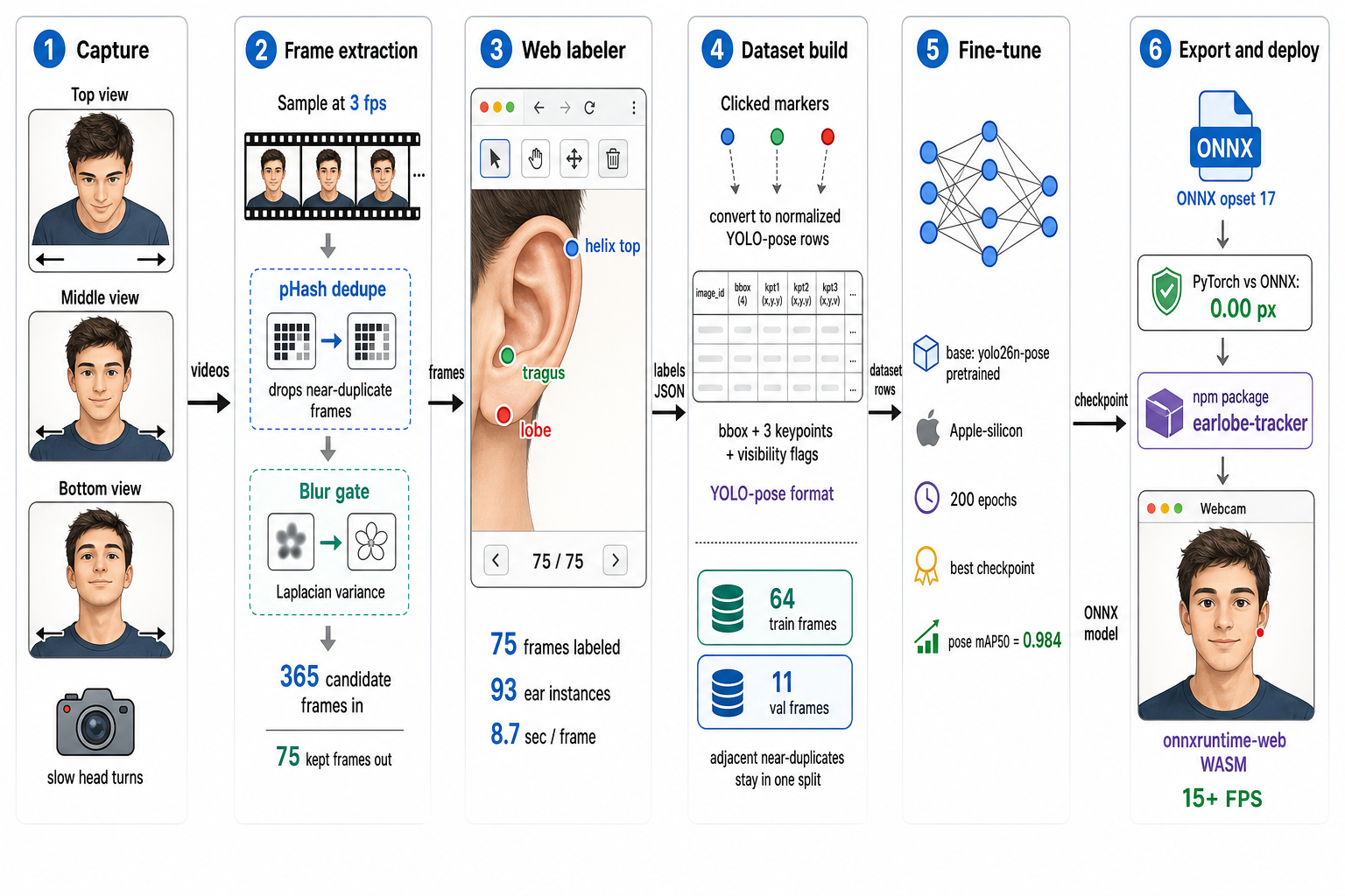
Design choices that matter more than they look:
- Deduplication is the sampling strategy. Frames are kept only if perceptually novel (dHash Hamming distance above 2) and sharp (Laplacian variance at least 40). A slow head sweep therefore yields exactly one frame per new pose, and redundant frames never inflate the dataset or the labeling bill.
- Time-block split instead of random split. Adjacent video frames are near-duplicates; a random train/val split would leak them across the boundary and inflate validation scores. Frames are split 85/15 in contiguous time blocks per video, so validation frames are genuinely unseen poses.
- A labeler built for this schema. A dependency-free web interface: click lobe → tragus → helix_top per visible ear, visibility flags, auto-expanded boxes. Three points per ear, because tragus and helix_top give the model ear structure to learn against; a lone pixel carries none.
drop at public/research/earlobe-tracker/media/labeler-session.mp4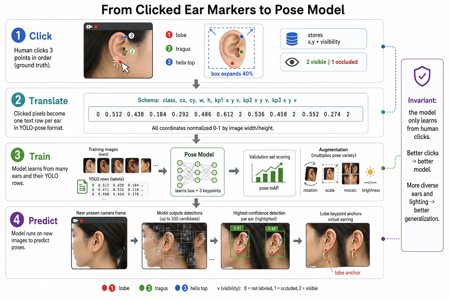
- The parity gate exists because export bugs are silent. A model that survives ONNX conversion with subtly wrong decode still runs; it's just wrong. Phase 5 re-runs the validation gallery through both runtimes and demands near-identical lobe coordinates.
What this run actually consumed (all measured)
| Quantity | Value | Source |
|---|---|---|
| Raw video | 3 clips: 43.7 s + 40.0 s + 38.0 s = 121.7 s total, 1620×1080 | file metadata |
| Frame candidates @ 3 fps | ≈ 365 | duration × rate |
| Frames kept after dedup + blur gate | 75 (top 30 · middle 19 · bottom 26) → ≈ 21% keep-rate | pipeline output |
| Labeled ear instances | 93 (1.24 per frame; 3 keypoints + visibility each) | label files |
| Labeling wall-time | 10.8 min for 75 frames ≈ 8.7 s/frame | label-file timestamps |
| Train / val | 64 / 11 frames, time-block split | dataset build |
Two minutes of video and eleven minutes of clicking. That is the entire data cost of everything that follows.
5 · The model
The pipeline explains how video becomes a checkpoint. This section is the model itself: what we started from, what the network actually is, and what fine-tuning changes.
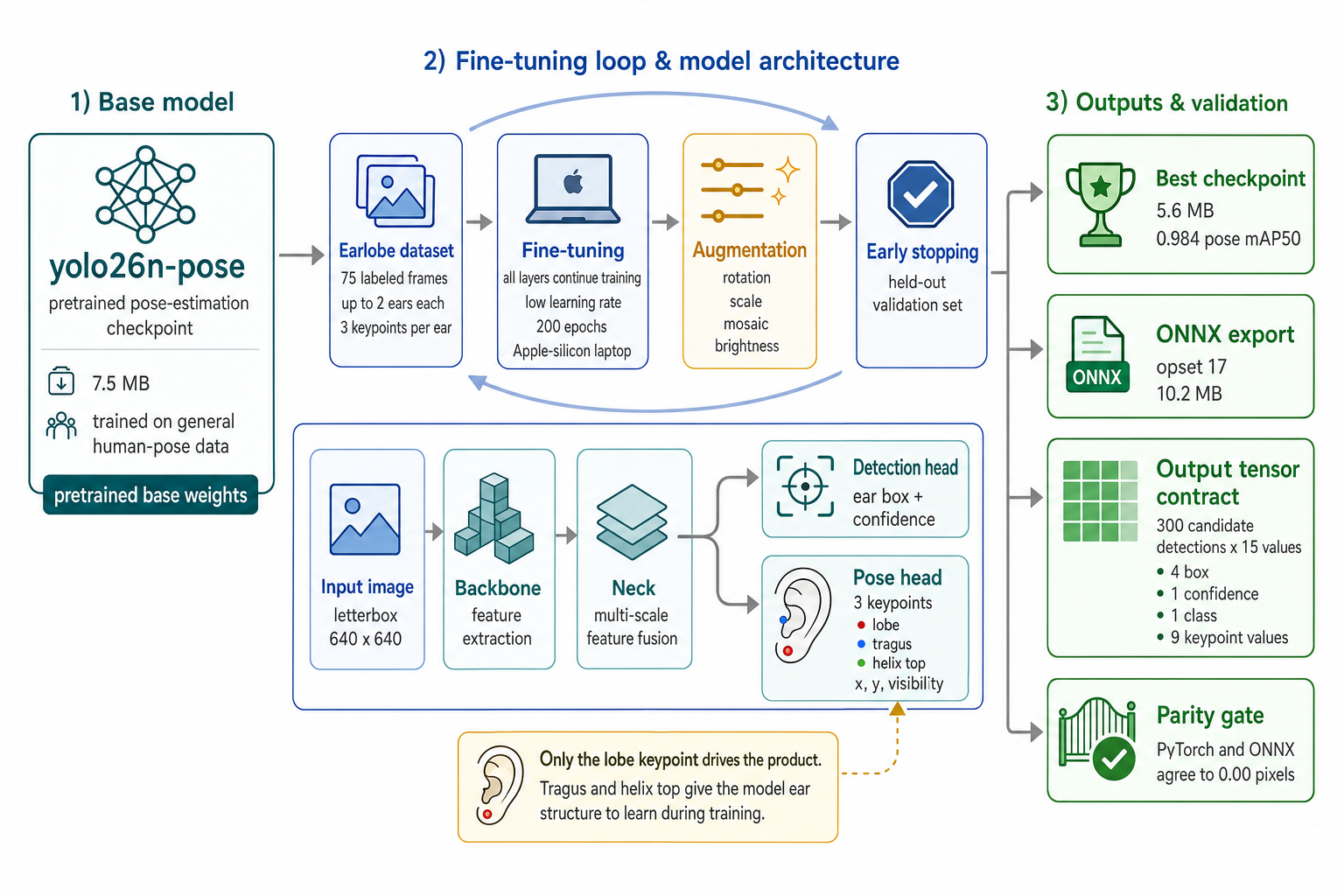
The base. We start from yolo26n-pose, a nano pose-estimation checkpoint (7.5 MB) pretrained on general human-pose data. That choice was a comparison, not a default:
| Candidate | Verdict |
|---|---|
| Train a keypoint network from scratch | Needs orders of magnitude more data than 75 frames, and there is nothing to transfer from. Ruled out. |
| MediaPipe / WebAR.rocks networks | Closed weights, no training lever at all. This is the original problem, not a solution to it. |
| Heatmap pose models (HRNet class) | Strong accuracy, but heavy for a mobile-browser WASM budget. |
| yolo26n-pose (chosen) | A pretrained pose head that transfers to a new keypoint schema on tiny data, nano-sized for the browser, exports cleanly to ONNX, and retrains with a config swap. |
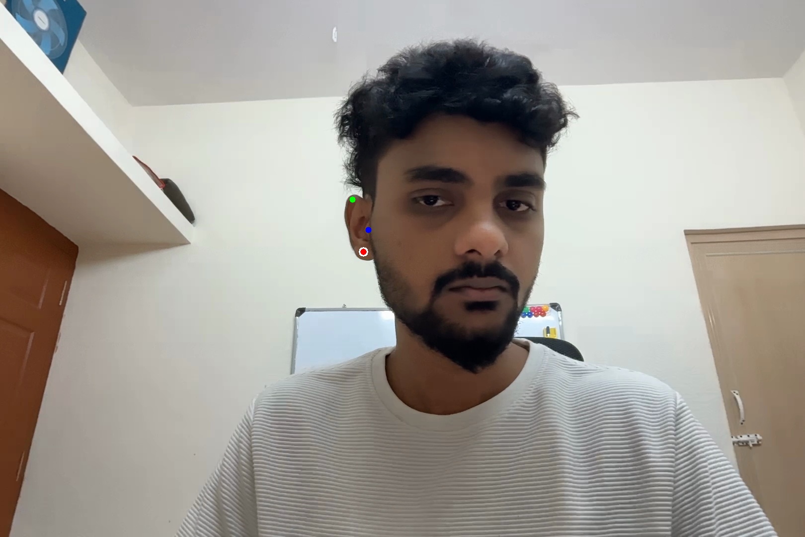
The network. The input frame is letterboxed to 640×640 and flows through a backbone (feature extraction), a neck (multi-scale fusion), and two heads side by side: a detection head that predicts the ear's bounding box and confidence, and a pose head that predicts the three keypoints, each carrying x, y, and a visibility score. The output is a single NMS-free tensor, [1, 300, 15]: 300 candidate detections of 15 values each (4 box, 1 confidence, 1 class, 9 keypoint values), with the lobe at columns 6 and 7.
What fine-tuning changes. All layers continue training at a low learning rate; nothing is frozen. The dataset is tiny, but the domain shift at the ear is real, and the augmentation policy carries the regularization load. Three keypoints are trained where the product needs one, because tragus and helix top give the network ear structure to learn against rather than a lone pixel.
6 · Results
Two training runs, both on a laptop (Apple-silicon MPS backend, no GPU server):
| v1.0 | v1.1 "hardened" | |
|---|---|---|
| Epoch budget | 150 (early-stop patience 50) | 200 (patience 60) |
| Epochs run | 112 | 103 |
| Wall time | 7.4 min | 39.4 min |
| Augmentation | mosaic 0.5 · ±10° · translate 0.10 · scale 0.3 | mosaic 0.6 · ±15° · translate 0.15 · scale 0.5 · hsv_v 0.5 (targeting motion blur & head tilt) |
| Checkpoint pose mAP50 | 0.9767 | 0.9844 (promoted) |
| Checkpoint pose mAP50-95 | — | 0.9781 |
Validation pose mAP50 per epoch for both runs, read mechanically from the runs' results.csv.
Validation pose loss per epoch. The hardened run trades a slower, noisier descent for robustness to motion blur and tilt.
Export integrity. The promoted checkpoint (5.6 MB PyTorch) exports to a 10.2 MB ONNX (opset 17, simplified, NMS-free [1, 300, 15] output with the lobe at columns 6–7). Re-running the validation gallery through PyTorch and ONNX Runtime produced lobe coordinates differing by 0.00 px. The parity gate passed with no measurable divergence.
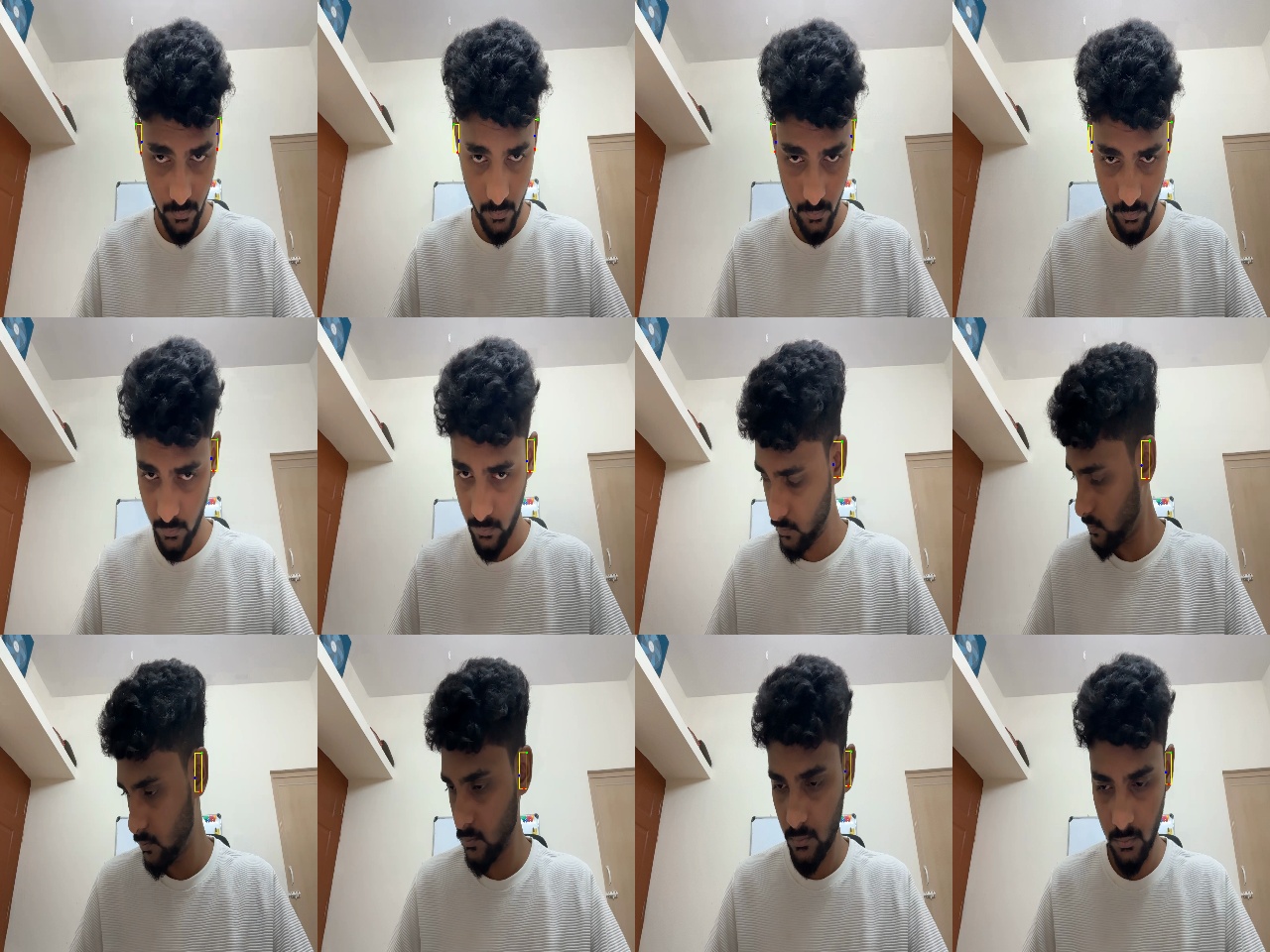
Browser runtime. The demo runs the ONNX model through onnxruntime-web (WebGPU where available, WebAssembly fallback) at ≥15 FPS on the development laptop under WASM, with One-Euro smoothing and velocity-predictive smoothing added after we observed motion trail on fast turns.
drop at public/research/earlobe-tracker/media/live-demo-wasm.mp4Packaging. The deliverable is a reusable module rather than a script:
import * as ort from "onnxruntime-web";
import { EarlobeTracker } from "earlobe-tracker";

const tracker = await EarlobeTracker.create({
  ort,
  modelUrl: "/earlobe.onnx",
  smoothing: true,
});
const { detections } = await tracker.detect(videoElement);
// detections: [{ lobe: { x, y }, conf, ... }]
ES module, zero hard dependencies (onnxruntime-web as peer), model shipped alongside, vanilla-JS and React examples included. It drops in beside the current production tracker (same conceptual output, one point per ear), which is what makes the rollout plan in §9 cheap.
Timeline. The repository's full history is five commits, all on one day: scaffold → pipeline + plumbing verification → real training run → reusable package → hardened retrain + motion-trail fix. Each phase closed its acceptance gate before the next began.
7 · Honest limits
- n = 1 by design. One subject, one camera, one room. The 0.984 figure is evidence for the pipeline; it says nothing about generalization.
- Expect the cliff. On the first diverse multi-person holdout, accuracy in the 0.70–0.75 mAP50 range would be normal for a single-subject fine-tune. This is the measurement that defines the data program. We plan for it up front instead of discovering it later.
- Small validation set. 11 frames / 16 instances: good enough to gate a pipeline, far too small to certify a product.
- No occlusion cases yet. Hair over ears, hands, existing jewellery: absent from the data, therefore unknown to the model.
None of these are flaws of the approach. They are the list of things data buys.
8 · What perfection costs
Everything below reuses the pipeline unchanged: one command per new video. The spec exists so the numbers are a decision instead of a guess. Measured anchors from this run are marked (m); projections are marked (est).
Capture protocol (per subject), standardized from what worked:
- 3 lighting conditions (low / mid / high) × 3 camera views (top / mid / bottom) × 2 platforms (web / mobile) = 18 videos
- Each a slow 5-minute sweep. Slow because deduplication keeps only novel poses (m: ≈ 21% keep-rate), so unhurried rotation maximizes unique-pose yield per minute; 5 minutes because this run's 40-second clips were the yield bottleneck
- ≈ 90 min recording ≈ 2 h session per subject including setup
Coverage. Subjects stratified by ear morphology (lobe attachment, size, helix shape; a short anthropometric taxonomy pass will fix the classes, expected 10–15, India-first sourcing with other-region top-up), plus age, gender, and skin-tone spread.
Yield & annotation (per subject): 18 × 5 min × 3 fps ≈ 16,200 candidates → ≈ 3,200 kept frames (est from the measured keep-rate). Labeling all of them is unnecessary; a stratified label budget of ~300 frames/subject (covering pose × lighting bins) is the recommended lever.
| Pilot | Solid | Production | |
|---|---|---|---|
| Subjects | 10 | 25 | 50+ |
| Recording sessions | 20 h | 50 h | 100 h (parallelizable) |
| Videos / footage | 180 / 15 h | 450 / 37.5 h | 900 / 75 h |
| Labeled frames (~300/subject) | 3,000 | 7,500 | 15,000 |
| Labeled ear instances (m: ×1.24) | ≈ 3,700 | ≈ 9,300 | ≈ 18,600 |
| Annotation, manual (m: 8.7 s/frame) | ≈ 7 h | ≈ 18 h | ≈ 36 h |
| Annotation, model-assisted (est: 2–3×) | ≈ 3 h | ≈ 7 h | ≈ 14 h |
| Single training run (est¹) | ~1–2 h GPU | ~3–5 h GPU | ~6–10 h GPU |
| Compute per tier incl. sweeps (est) | under $50 | ~$100–200 | ~$150–300 |
¹ Anchored to the measured laptop run (64 images / 200 epochs / 39.4 min on MPS), extrapolated to a single cloud GPU; refine after the first cloud run.
Annotation quality. The web labeler already supports the workflow; add a 10% double-label spot-check, and switch to model-assisted pre-labeling (the current model proposes, a human corrects) as soon as the pilot model exists. That is where the 2–3× comes from.
Evaluation gate for promotion. Stratified holdout by subject, ear type, lighting, and view; report per-stratum mAP and pixel error at the lobe; a candidate model is promoted only if no stratum regresses. This is the production version of the parity-gate discipline applied at export time in this run.
9 · Rollout
- Shadow mode. Ship the package alongside the current tracker; log both anchors per frame; zero user-facing change.
- Offline comparison. Replay captured sessions; measure disagreement distribution and per-stratum pixel error against spot-truth.
- Gated A/B. Swap the anchor source behind a flag for a slice of sessions; watch the physics stability metrics (rest jitter at the pin) as the product-level signal.
- Promote or iterate. The npm API was shaped so this whole sequence turns on data, with no integration project attached.
10 · Conclusion
The expensive question (is a custom, in-browser, lobe-specific tracker feasible without a research team?) is now answered with a working artifact rather than an opinion: a versioned pipeline, gates that caught real bugs, a 0.984-mAP50 checkpoint from two minutes of video, a 0.00 px export parity, and a package that drops in beside production. What remains is no longer research: a data-collection program with a measured cost per unit of accuracy. This note is its specification.
Appendix
A. ONNX I/O contract. Input images [1,3,640,640] float32, letterboxed. Output output0 [1,300,15] float32, confidence-sorted, NMS-free. Column map: x1, y1, x2, y2, conf, class, lobe_x, lobe_y, lobe_v, tragus_x, tragus_y, tragus_v, helix_x, helix_y, helix_v. The letterbox inverse (scale, pad_x, pad_y) maps coordinates back to source pixels.
B. Keypoint schema. Per ear instance: lobe, tragus, helix_top, each (x, y, v) with v = 1 occluded-but-placed or v = 2 visible; bbox auto-expanded +40% around the points; identity flip index (no left/right symmetry within an ear); single class, "ear".
C. Environment. Python 3.11 · torch 2.12.1 · ultralytics 8.4.87 · onnx 1.22.0 · onnxruntime 1.27.0 · onnxruntime-web 1.22.0 (vendored WASM) · training device: Apple-silicon MPS with a loss-sanity guard (NaN/zero → CPU fallback).
D. Reproduce. Setup → frames → label (human) → dataset → train → export → demo, each a single make target; a chained target runs the non-human phases; a synthetic smoke target proves the plumbing end-to-end before any real video exists.
E. Data provenance. All measured figures in this note are read mechanically from the run's artifacts: the runs' results.csv (training curves), the pipeline's metrics.json (promoted checkpoint), onnx_io.json (I/O contract), label-file timestamps (annotation rate), and video container metadata (durations). The extraction scripts and staged source reports live beside this document in the project repository.